Making Sense of the Weird Spatial Twist

If you are learning robot kinematics, you will often work with a frame attached to a rigid body. The frame has position $p(t)$ and orientation $R(t)$ in the world frame $W$. Its origin moves with velocity $\dot p$, and the body has angular velocity $\omega$.

To describe translation and rotation together, we use a six-dimensional velocity vector called a twist. You might expect to build it simply by stacking $\omega$ and $\dot p$:

$$\begin{bmatrix} \omega\ \dot p \end{bmatrix}.$$

Then you open a textbook such as Modern Robotics (Section 3.3.2) and encounter the definition of a spatial twist:

$$V^W = \begin{bmatrix} \omega\ \dot p-\omega\times p \end{bmatrix}.$$

Why subtract $\omega\times p$? Isn’t $\dot p$ already the linear velocity expressed in the world frame?

You read on. The textbook asks you to imagine extending the moving body to infinite size, then describes the linear part as:

“the instantaneous velocity of the point on this body currently at the fixed-frame origin, expressed in the fixed frame”

— Lynch and Park, Modern Robotics, Section 3.3.2, p. 97

Wait. You started with a perfectly ordinary rigid body. Now, just to make sense of its “linear velocity,” you have to imagine extending it to infinity and pick out the material point on that imaginary extension that happens to pass through the world origin. All this when $\dot p$ already tells you how the frame origin is moving. Why go to all this trouble?

Describing the Body’s Motion

The answer is: we want to describe the motion of the rigid body, independent of how we attach the frame.

Why does that matter, you might ask? With $\dot p$, we could report different “linear velocities” for the very same rigid-body motion, just by choosing different places to attach a frame. More importantly, this representation lets us combine the motions of connected rigid bodies. For a robot arm, that means adding up the contributions of its links to get the end-effector’s motion. We’ll see that in a moment. But first, let’s see why this correction works.

Keeping the world frame fixed, call the body frame’s origin $P$ and pick any point fixed to the body, at world position $x$. Draw an arrow $r$ from $P$ to that point, expressed in world coordinates.

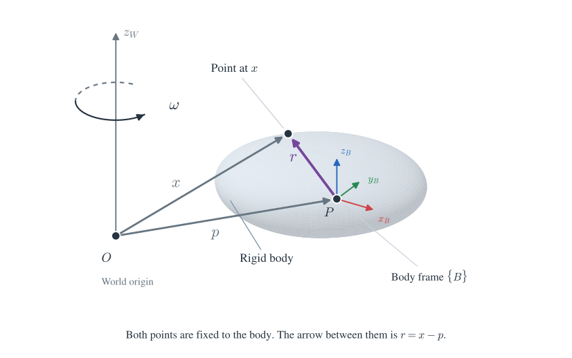
The arrows give

$$x=p+r.$$

Differentiating both sides, and using $\dot r=\omega\times r$ because $r$ rotates with the body, gives

$$\dot x=\dot p+\dot r=\dot p+\omega\times r.$$

Substitute $r=x-p$ and collect the terms that depend on $x$:

$$\dot x=\omega\times x+(\dot p-\omega\times p).$$

Keep your eye on the same point at $x$. At this same instant, imagine choosing a different origin for the body frame. The point’s velocity $\dot x$ hasn’t changed, and neither has $\omega\times x$. So the remaining term, $\dot p-\omega\times p$, must stay the same, even though $p$ and $\dot p$ may change.

Adding Motion Along a Chain

The formula above describes a velocity field: at any location $x$, it tells us how fast a point attached to the body would move there. This is an Eulerian view of motion: we choose a fixed location in space and observe the motion there. Evaluating the velocity at the world origin, $x=0$, gives

$$\left.\dot x\right|_{x=0} =\omega\times 0+(\dot p-\omega\times p) =\dot p-\omega\times p.$$

The textbook’s infinitely large extension is just a way to picture this velocity field beyond the physical body. Asking for the velocity of the imaginary material point passing through the world origin is simply evaluating the field at $x=0$. Together with the angular velocity $\omega$, this gives us the spatial twist.

Now connect several rigid bodies into a robot arm. Each link’s motion relative to its parent contributes its own velocity field. Express these contributions in the same world frame, and their linear parts are all evaluated at the same spatial location. We can add those velocities, together with the angular velocities, to get the end-effector’s twist.

Consider a planar two-link arm with each link $1,\mathrm{m}$ long. At this instant, the first link points along the world $x$-axis and the elbow is bent by $90^\circ$, so the second link points along $y$. The shoulder, at the world origin, turns at $+1,\mathrm{rad/s}$ about $z$. The elbow turns at $-1,\mathrm{rad/s}$ relative to the first link.

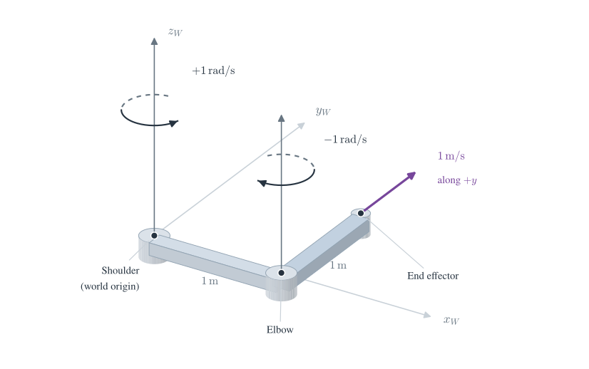
To find each contribution, let that joint move while holding the other joint fixed:

• The shoulder rotates the entire arm about the world origin, so its twist has zero linear part.
• The elbow rotates the second link about the elbow. For this contribution, the elbow point is stationary, but it is one metre along $x$ from the world origin. The correction $-\omega\times p$ gives a linear part of $+1,\mathrm{m/s}$ along $y$.

Adding the two contributions gives the end-effector twist:

$$V^W_{\mathrm{ee}} = \underbrace{\begin{bmatrix}0\0\1\0\0\0\end{bmatrix}}$${\text{shoulder}} + \underbrace{\begin{bmatrix}0\0\-1\0\1\0\end{bmatrix}}{\text{elbow}} = \begin{bmatrix}0\0\0\0\1\0\end{bmatrix}.

The end effector has zero angular velocity but still moves at $1,\mathrm{m/s}$ along $y$. For a longer chain, we keep adding each joint’s contribution in the same world frame.

(This also gives us a clean geometric derivation of the space Jacobian.)

World Velocity in Code

We now have good reasons to prefer the textbook’s definition, despite how odd it first looked: it describes the body’s motion independently of where we attach the frame, and lets us combine the motions of connected bodies by simple addition.

Unfortunately, robotics libraries do not all follow this convention when reporting “world velocity.” MuJoCo’s site-velocity query, for example, returns the site’s ordinary point velocity as its linear part. Pinocchio’s WORLD query follows the textbook definition.

Return to the frame at $P$ in our first diagram and put in some numbers. At one instant, let

$$p=\begin{bmatrix}1\0\0\end{bmatrix},\mathrm{m}, \qquad \dot p=\begin{bmatrix}0\1\0\end{bmatrix},\mathrm{m/s}, \qquad \omega=\begin{bmatrix}0\0\1\end{bmatrix},\mathrm{rad/s}.$$

Place a MuJoCo site and a Pinocchio frame at $P$, with both models evaluated at this state. Both queries use world axes:

velocity = np.zeros(6)
mujoco.mj_objectVelocity(
    mj_model, mj_data, mujoco.mjtObj.mjOBJ_SITE,
    site_id, velocity, 0,  # use world axes
)
print(velocity[3:])  # MuJoCo stores [angular; linear].
# [0. 1. 0.]

WORLD = pin.ReferenceFrame.WORLD
print(pin.getFrameVelocity(model, data, frame_id, WORLD).linear)
# [0. 0. 0.]

MuJoCo’s site query returns $\dot p$, the velocity at $P$. Pinocchio’s WORLD query returns $\dot p-\omega\times p$, which is zero for these numbers. Both report the same angular velocity $\omega$. The difference is exactly the choice of reference point we just worked through.

Keeping the Origin at the Body

But if our original definition was “wrong,” why does MuJoCo use it?

There was nothing wrong with $\dot p$. Suppose your robot arm is picking up an object from a moving conveyor. Before closing the gripper, you want its grasp point $P$ to move with the object. That means matching $\dot p$ to the object’s velocity. MuJoCo’s site query gives us exactly this velocity at $P$.

So how do we get the same point velocity from Pinocchio? Picture a coordinate frame whose origin follows $P$, while its axes stay parallel to the world axes even as the body turns. This is what Pinocchio calls LOCAL_WORLD_ALIGNED, or LWA.

Putting the origin at $P$ removes the offset responsible for the $-\omega\times p$ term. Keeping the axes world aligned gives us $\dot p$ in world coordinates. We are still describing the body’s motion relative to the world, so the angular component remains the body’s $\omega$:

$$V^{\mathrm{LWA}} = \begin{bmatrix} \omega\ \dot p \end{bmatrix}.$$

Changing the query to LWA gives

LWA = pin.ReferenceFrame.LOCAL_WORLD_ALIGNED
print(pin.getFrameVelocity(model, data, frame_id, LWA).linear)
# [0. 1. 0.]

Now the results agree: both queries give the velocity at $P$, expressed in world axes.

We’ve finally made sense of velocity. But to take the next step from kinematics to dynamics, we need acceleration too. Surely that just means differentiating the velocity?

Yet ask MuJoCo and Pinocchio for acceleration at the same point, using the same world axes, and they can disagree all over again. We’ll see why in the next post.